Chapter III: Preferences and Investor Choice

An Introduction to Investment Theory

© William N. Goetzmann
YALE School of Management

Chapter III: Preferences and Investor Choice

The last chapter presented the Markowitz model of portfolio selection, but with one key element missing -- individual portfolio choice. The efficient frontier dominates all combinations of assets, however it still has infinitely many assets. How do you pick one portfolio out of all the rest as the perfect one for you? This turns out to be a big challenge, because it requires investors to express their preferences in risk-return space. Investors choose portfolios for a myriad of reasons, very few of which can be reduced to a two-dimensional space. In fact, investors are used to having the ability the CHANGE their investment decision if it is not developing as planned. The simple Markowitz model does not allow this freedom. It is a single period model, now used widely in practice for decision-making in a multi-period world. In this chapter, we will address some of the ways that one may approximate investor preferences in mean-variance space, however these methods are only approximations.

I. Choosing A Single Portfolio

How might you choose a single portfolio among all of those on the efficient frontier? One approach is to model investor preferences mathematically, using iso-utility curves. These curves express the risk-return trade-off for investors in two-dimensional space. They work exactly like lines on a topological map. They are nested lines that show the highest and lowest altitudes in the region -- except they measure altitude in units of utility (whatever that is!) instead of feet or meters. Typically, a convenient mathematical function is chosen as the basis for iso-utility curves. For instance, one could use a logarithmic function, or even part of a quadratic function to capture the essence of investor preferences. The essential feature of the function is that it must allow people to demand ever-increasing levels of return for assuming more risk.

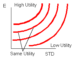
Although the mathematics of utility functions is beyond the scope of this course, if you are interested in further investigation, I recommend visiting Campbell Harvey's Pages on Optimal Portfolios.

One way to characterize differences in investor risk aversion is by the curvature of the iso-utility lines. Below are representative curves for four different types of investors: A more risk-averse, a moderately risk-averse, a less risk-averse, and a risk-loving investor. The whole set of nested curves is omitted to keep the picture simple.

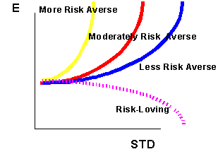
Notice that the risk-lover demands lower expected return as risk increases in order to maintain the same utility level. On the other hand, for the more risk-averse investor, as volatility increase, he or she will demand sharply higher expected returns to hold the portfolio. These different curves will result in different portfolio choices for investors. The optimization procedure simply takes the efficient frontier and finds its point of tangency with the highest iso-utility curve in the investor set. In other words, it identifies the single point that provides the investor with the highest level of utility. For risk-averse individuals, this point is unique.

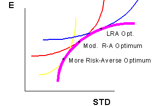
The problem with applying this methodology to identifying optimal portfolios is that it is difficult to figure out the risk-aversion of individuals or institutions. Just like mapping an unknown terrain, the asset allocator must try to map the clients preference structure -- never knowing whether it is even consistent from one day to the next!

II. Another Approach: Preferences about Distributions

The Markowitz model is an elegant way to describe differences in distributions of returns among portfolios. One approach to the portfolio selection problem is to choose investment policies based upon the probability mass in the lower left-hand tail. This is called the short-fall criterion. It's simplicity has great appeal. It does not require a complete topological mapping of investor preferences. Instead it only requires the investor to specify a floor return, below which he or she wants to avoid falling. The short-fall approach chooses a portfolio on the efficient frontier that minimizes the probability of the return dropping below that floor. Suppose, for instance, your specify a floor return level equal to the riskless rate, R_f. For every portfolio on the frontier, you calculate the ratio:

Notice that the shortfall criterion is like a t-statistic, where the higher the value, the greater the probability. The portfolio that has the highest probability of exceeding R_f is the one for which this value is maximized. In fact, the similarity to a t-statistic extends even further, as we will see.

Another useful thing is that it turns out that it is quite simple to find the portfolio that maximizes the probability of exceeding the floor. You can do it graphically!

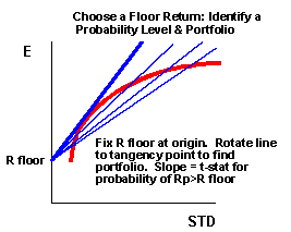
Identify the floor return level on the Y axis. Then find the point of tangency to the efficient frontier. In the figure, for instance, the tangency point minimizes the probability of having a return that drops below R floor. One particular floor value is of interest -- that is the floor given by the riskless rate, R_f. The slope of the short-fall line when R_f is the floor is called the Sharpe Ratio. The portfolio with the maximum Sharpe Ratio is the one portfolio in the economy that minimizes the probability of dropping below treasury bills. By the same token, it is the one portfolio in the economy that has the maximum probability of providing an equity premium! That is, if you must bet on one portfolio to beat t-bills in the future, the tangency portfolio found via the Sharpe Ratio would be it.

The "safety-first" approach is a versatile one. In the above example, we maximized probability of exceeding a floor by maximizing the slope, identifying a point of tangency. You can also find portfolios by other methods. For instance, you can check the feasibility of a desired floor and probability of exceeding that floor by fixing the Y intercept and fixing the slope. Either the ray will pass through the feasible set, or it will not. If it does not, then there is no portfolio that meets the criteria you specified. If it does, then there are a number of such portfolios, and typically the one with the highest expected return is the one to choose.

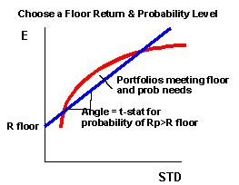
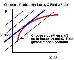
Another approach is to find a floor that meets your probability needs. In other words, you ask "Which floor return may I specify that will give me a 90% confidence level that I will exceed it?" This is equivalent to setting the slope equal to the t-statistic value matching that probability level. Since this is equivalent to a one-tailed test, you would set the slope to 1.28 (i.e. the quantile of the normal distribution that gives you 90% to the left, or 10% in the right side of the distribution. For a 95% chance, you would choose a slope of 1.644. For a 99% chance you would choose a slope of 2.32.

Once you choose the slope, then move the line vertically until it becomes a tangent. This will give you both a floor and a portfolio choice.

III. A Note on Value at Risk

The safety first approach can be used to calculate the value-at-risk of the portfolio. Value-at-risk is an increasingly popular measure of the potential for loss over a given time horizon. It is applied in the banking industry to calculate capital requirements, and it is applied in the investment industry as a risk control for portfolios of securities.

Consider the problem of estimating how big a loss your portfolio could experience over the next month. If the distribution of portfolio returns is normal, then a three standard deviation drop is possible, but not very likely. Typically, the estimate of the maximum expected loss is defined for a given time horizon and a given confidence interval. Consider the type of loss that occurs once in twenty months. If you know the mean and standard deviation of the portfolio, and you specify the confidence interval as a 5% event (1 in twenty months) or a 1% event (1 in a hundred months) it is straightforward to calculate the "Value at Risk."

Let Rp be the portfolio return and STDp be the portfolio standard deviation. Let T be the t-statistic associated with the confidence interval. T of 1.64 corresponds to a one in 20 month event. Let Rvar be the unknown negative return portfolio return that we expect to occur one in twenty times.

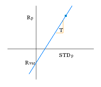
The equation for the line is: Rp = Rvar + T*STDp and thus, Rvar = Rp - T*STDp. Rvar multiplied times the value of the assets in the portfolio is the Value at Risk.

Suppose you are considering the VAR of a $100 million pension portfolio over the monthly horizon. It is composed of 60% stocks and 40% bonds, and you are interested in the 95% confidence interval.

Let us assume that the monthly expected stock return is 1% and the expected bond return is .7%, and their standard deviations are 5% and 3% respectively. Assume that the correlation between the two asset classes is .5. First we calculate the mean and standard deviation of the portfolio:

Rp = (.6)*(.01) + (.4)(.007) = .0088

STDp = sqrt[ .6^2.05^2 + .4^2.03^2 + 2.5.6.4.05*.03] = .038

Then, Rvar = .0088 - 1.64*.038 = -.054

Thus, the monthly value-at-risk of the portfolio is ($100 million)(.054) = $5.4 million.

Note that, despite the terminology, this does not really mean that $94.6 is not at risk. The analysis only means that you expect a loss at least as large as $5.4 million one month out of 20.

This approach to calculating value-at-risk depends on key assumptions. First, returns must be close to normally distributed. This condition is often violated when derivatives are in the portfolio. Second, historically estimated return distributions and correlations must be representative of future return distributions and correlations. Estimation error can be a big problem when you have statistics on a large number of separate asset classes to consider. Third, returns are not assumed to be auto-correlated. When there are positive trends in the data, losses should be expected to mount up from month to month.

In summary, value at risk is becoming pervasive in the financial industry as a summary measure of risk. While it has certain drawbacks, its major advantage is that it is a probability-based approach that can be viewed as a simple extension of safety-first portfolio selection models.

IV. Conclusion

Creating an efficient frontier from historical or forecast statistics about asset returns is inherently uncertain due to errors in statistical inputs. This uncertainty is minor when compared to the problem of projecting investor preferences into mean-standard deviation space. Economists know relatively little about human preferences, especially when they are confined to a single-period model. We know people prefer more to less, and we know most people avoid risk when they are not compensated for holding it. Beyond that is guess-work. We don't even know if they are consistent, through time, in their choices. The theoretical approach to the portfolio selection problem relies upon specifying a utility function for the investor, using that to identify indifference curves, and then finding the highest attainable utility level in the feasible set. This turns out to be a tangency point. In practice, it is difficult to estimate a utility function, and even more difficult to explain it back to the investor.

An alternative to utility curve estimation is the "safety-first" technology, which is motivated by a simple question about preferences. What is your "floor" return? If you can pick a floor, you can pick a portfolio. In addition, you can identify a probability of exceeding that floor, by observing the slope of the tangency line. Safety-first also lets you find optimal portfolios by picking a floor and a probability, as well as simply picking a probability.

Value at risk is becoming increasingly popular method of risk measurement and control. It is a simple extension of the safety-first technology, when the assets comprising the portfolio have normally distributed returns.

IV. Epilogue

Notice that the introduction of a genuine risk-free security simplifies the portfolio problem for all investors in the world. Their optimal choice is reduced to the problem of choosing proportions of the riskless asset and the risky portfolio T (tangency). MRA (More Risk Averse) investors will hold a mix of tangency portfolio and T-bills, LRA (Less Risk Averse) investors will borrow at the riskless rate and invest the proceeds in the tangency portfolio.

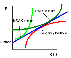
If we could only figure out what the tangency portfolio is composed of, we could solve everyone's investment decision with the same product! What do you think T is composed of? The answer is in the next chapter.

For more information about the utility approach to risk, see the excellent write-up by Campbell Harvey on Optimal Portfolios.. For a comprehensive hyper-text book on investment decision-making, see William Sharpe's Macro-Investment Analysis

An Introduction to Investment Theory