Chapter II: The Geography of the Efficient Frontier

An Introduction to Investment Theory

© William N. Goetzmann
YALE School of Management

Chapter II: The Geography of the Efficient Frontier

In the previous chapter, we saw how the risk and return of investments may be characterized by measures of central tendency and measures of variation, i.e. mean and standard deviation. In fact, statistics are the foundations of modern finance, and virtually all the financial innovations of the past thirty years, broadly termed "Modern Portfolio Theory," have been based upon statistical models. Because of this, it is useful to review what a statistic is, and how it relates to the investment problem. In general, a statistic is a function that reduces a large amount of information to a small amount. For instance, the average is a single number that summarizes the typical "location" of a set of numbers. Statistics boil down a lot of information to a few useful numbers -- as such, they ignore a great deal. Before modern portfolio theory, the decision about whether to include a security in a portfolio was based principally upon fundamental analysis of the firm, its financial statements and its dividend policy. Finance professor Harry Markowitz began a revolution by suggesting that the value of a security to an investor might best be evaluated by its mean, its standard deviation, and its correlation to other securities in the portfolio. This audacious suggestion amounted to ignoring a lot of information about the firm -- its earnings, its dividend policy, its capital structure, its market, its competitors -- and calculating a few simple statistics. In this chapter, we will follow Markowitz' lead and see where the technology of modern portfolio theory takes us.

I. The Risk and Return of Securities

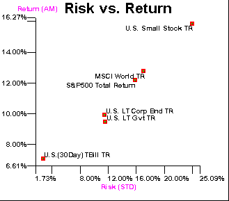
Markowitz's great insight was that the relevant information about securities can be summarized by three measures: the mean return (taken as the arithmetic mean), the standard deviation of the returns and the correlation with other assets' returns. The mean and the standard deviation can be used to plot the relative risk and return of any selection of securities. Consider six asset classes:

(Courtesy Ibbotson Associates)

This figure was constructed using historical risk and return data on Small Stocks, S&P stocks, Corporate and Government Bonds, and an international stock index called MSCI, or Morgan Stanley Capital International World Portfolio. The figure shows the difficulty an investor faces about which asset to choose. The axes plot annual standard deviation of total returns, and average annual returns over the period 1970 through 3/1995. Notice that small stocks provide the highest return, but with the highest risk. In which asset class would you choose to invest your money? Is there any single asset class that dominates the rest? Notice that an investor who prefers a low risk strategy would choose T-Bills, while an investor who does not care about risk would choose small stocks. There is no one security that is best for ALL investors.

II. Portfolios of Assets

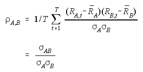
Typically, the answer to the investment problem is not the selection of one asset above all others, but the construction of a portfolio of assets, i.e. diversification across a number of different securities. The key to diversification is the correlation across securities. Recall from data analysis and statistics that the correlation coefficient is a value between -1 and 1, and measures the degree of co-movement between two random variables, in this case stock returns. It is calculated as:

Where the sigma AB is the covariance of the two securities. Here is how to use correlation in the context of portfolio construction. Consider two securities, A and B. Security A has a mean of 10% and an STD of 15%. Security B has a mean of 20% and an STD of 30%. We can calculate the standard deviation of a portfolio composed of different mixtures of A & B using this equation:

The mean return is not as complicated. It is a simple weighted average of the means of the two assets:
mean _p = W _A R_A + W _B R _B. Notice that a portfolio will typically have a weight of one, so usually, W _A + W _B = 1.

What if the correlation of A&B = 0 ? Notice that a portfolio of 80% A and 20% B has a standard deviation of: sqrt(.8²*.15²+.2².3²+2*0*.8*.2*.15*.3) = 13.4 %

In other words, a mixture of 20% of the MORE RISKY SECURITY actually decreases the volatility of the portfolio! This is a remarkable result. It means you can reduce risk and increase return by diversifying across assets.

What if the correlation of A&B = 1 ? In this case, the perfect correlation between the two assets means there is no diversification. The portfolio std of of the 80/20 mix is 18%. this is equal to a linear combination of the standard deviations: (.8)(.15)+(.2)(.30) = 18%

What if the correlation of A&B = -1 ? This is an unusual case, because it means that when A moves up, B always moves down. Take a mixture of .665 A and (1-.665) B. sqrt(.665²*.15²+(1-.665)².3²+2*0*(.665)*(1-.665)*.15*.3) = .075%, Which is very close to zero. In other words, A is nearly a perfect hedge for B. One of the few real-life negative correlations you will find is a short position in a stock offsetting the long position. In this case, since the mean returns are also the same, the expected return will be zero. These extremes of correlation values allow us to describe an envelope within which all combinations of two assets will lie, regardless of their correlations.

(Courtesy Campbell Harvey)

III. More Securities and More Diversification

Now consider what will happen as you put more assets into the portfolio. Take the special case in which the correlation between all assets is zero, and all of them have the same risk. You will find that you can reduce the standard deviation of the portfolio by mixing across several assets rather than just two. Each point represents an equally-weighted combination of assets; from a single stock to two, to three, to thirty, and more. Notice that, after 30 stocks, diversification is mostly achieved. There are enormous gains to diversification beyond one or two stocks.

(Courtesy Campbell Harvey)

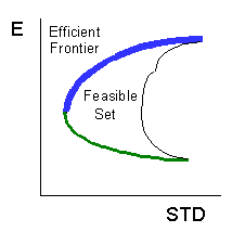
If you allow yourself to vary the portfolio weights, rather than keeping them equal, the benefits are even greater, however the mathematics is more challenging. You not only have to calculate the STD of the mixture between A&B, but the STD of every conceivable mixture of the securities. None-the-less, If you did so, you would find that there is a set of portfolios which provide the lowest level of risk for each level of return, and the highest level of return for each level of risk. By considering all combinations of assets, a special set of portfolios stand out -- this set is called the efficient frontier.

The efficient frontier, shown in blue, is the set of dominant portfolios, at least from the perspective of a risk averse investor. For ANY level of risk, the efficient frontier identifies a point that is the highest returning portfolio in its risk class. By the same token, for any level of return, the frontier identifies the lowest risk portfolio in that return class. Notice that it extends from the maximum return portfolio (actually a single asset) to the minimum variance portfolio. The efficient frontier has a portfolio for everyone -- there are an infinite number of points in the set, corresponding to the infinite variation in investor preferences for risk. The area called the feasible set represents all feasible combinations of assets. There are no assets that fall outside of the feasible set.

IV. Markowitz and the First Efficient Frontier

The first efficient frontier was created by Harry Markowitz, using a handful of stocks from the New York Stock Exchange. Here it is, reproduced from his book Portfolio Selection Cowles Monograph 16, Yale University Press, 1959. It has a line going to the origin, because Markowitz was interested in the effects of combining risky assets with a riskless asset: cash.

Notice, too, that it is tipped on its side. The convention of STD on the X axis is developed later.

V. An Actual Efficient Frontier Today

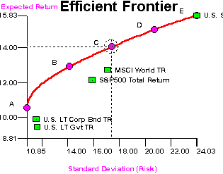
This figure is an efficient frontier created from historical inputs for U.S. and international assets over the period 1970 through 3/1995, using the Ibbotson EnCorr Optimizer program.

(Courtesy Ibbotson Associates)

This is state-of-the-art portfolio selection technology, however it is still based upon Markowitz's original optimization program. There are some basic features to remember:

A minimum variance portfolio exists
A maximum return portfolio is composed of a single asset.
B,C,D & E are critical points at which one the set of assets used in the frontier changes, i.e. an asset drops out or comes in at these points.
There are no assets to the northwest of the frontier. That is why we call it a frontier. It is the edge of the feasible combinations of risk and returns.

VI. The Efficient Frontier with the Riskless Asset

T-Bills are often taken to be riskless assets, and their return is indicated as R_f, the risk-free rate. Once you allow the riskless asset to be combined into a portfolio, the efficient frontier can change. Since it is riskless, it has no correlation to other securities. Thus it provides no diverisfication, per se. It does provide an opportunity to have a low-risk portfolio, however. This picture is a diagram of the efficient frontier composed of ALL the risky assets in the economy, as well as the riskless asset.

(Courtesy Campbell Harvey)

In this special case, the new efficient frontier is a ray, extending from R_f to the point of tangency (M) with the "risky-asset" efficient frontier, and then beyond. This line is called the Capital Market Line (CML). It is actually a set of investable portfolios, if you were able to borrow and lend at the riskless rate! All portfolios between R_f and M are portfolios composed of treasury bills and M, while all portfolios to the right of M are generated by BORROWING at the riskless rate R_f and investing the proceeds into M.

VII. Summary

The Markowitz model was a brilliant innovation in the science of portfolio selection. With almost a disarming slight-of-hand, Markowitz showed us that all the information needed to choose the best portfolio for any given level of risk is contained in three simple statistics: mean, standard deviation and correlation. It suddenly appeared that you didn't even need any fundamental information about the firm! The model requires no information about dividend policy, earnings, market share, strategy, quality of management -- nothing about the myriad of things with which Wall Street analysts concern themselves! In short, Harry Markowitz fundamentally altered how investment decisions were made. Virtually every major portfolio manager today consults an optimization program. They may not follow its recommendations exactly, but they use it to evaluate basic risk and return trade-offs.

Why doesn't everyone use the Markowitz model to solve their investment problems? The answer again lies in the statistics. The historical mean return may be a poor estimate of the future mean return. As you increase the number of securities, you increase the number of correlations you must estimate -- and you must estimate them CORRECTLY to obtain the right answer. In fact, with more than 1,500 stocks on the NYSE, one is certain to find correlations that are widely inaccurate. Unfortunately, the model does not deal well with incorrect inputs. That is why it is best applied to allocation decisions across asset classes, for which the number of correlations is low, and the summary statistics are well estimated.